Autonomous Driving Robot
Practicing:
- Project Management and Advanced Problem Solving
- Rapid Prototyping, Manufacturing (machine shop) and CAD
- Soldering, Electronics and PCB Design
- Troubleshooting (noise issues, signal integrity, software and hardware)
Pictures:
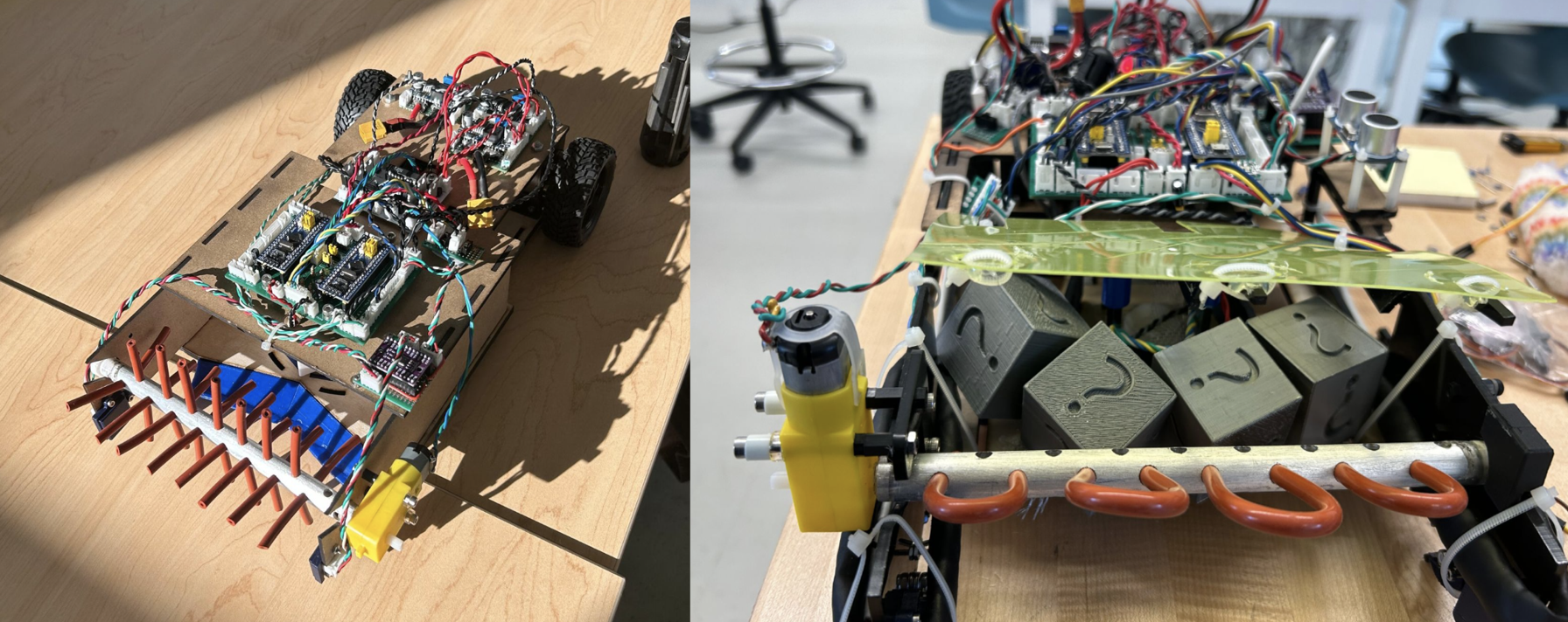
Some History and Outline:
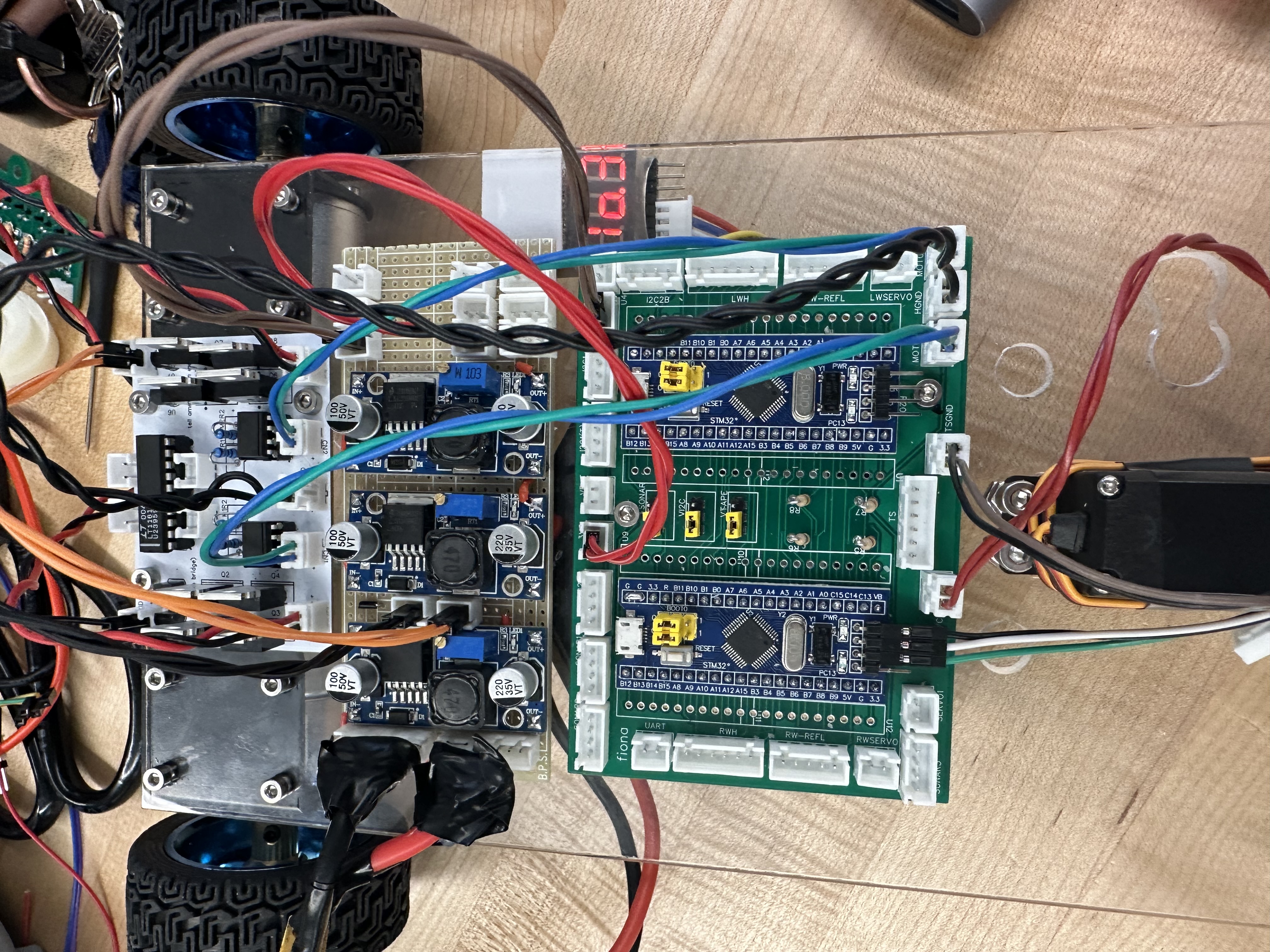
Over the 2023 Summer Term from July 4 to August 10, myself, Ebrahim Hussain, Amr Sherif, and Dhruv Arun came together in a team of 4 for the annual ENPH 253 robot competition. The final robot photos above represent all of our unique contributions and our less than straightforward path which led us to our final design. This post highlights our conceptual ideas, decisions, and the manufacturing of our robot. We concluded the term with a 2nd-place finish.
- The full race can be watched here.
The Track:
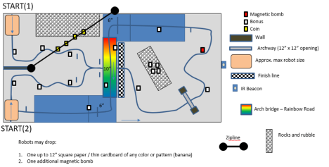
Summary of Rules:
- Heats are 2 minutes long.
- Robots score points by picking up prize blocks (labelled “Bonus”) on the track, coins (labelled “Coin”) on the zipline, or by completing a lap. Blocks and coins are worth 1 point each, while a lap is worth 3.
- Regardless of START(1) or START(2), a lap is counted when a robot completes the following in order:
- Crosses over the finish line.
- Goes up the ramp (blue, top right) and either jumps down on the left side of Rainbow Road or loops around to START(2).
- Travels under Rainbow Road from the left and crosses the finish line again.
- A magnetic “bomb” is placed on the track, which has the same footprint as a regular Bonus/prize block. Each robot is also allowed to drop one extra bomb on the track at any time throughout the heat.
- Any robot that picks up a bomb or tips it on its side has “detonated” the bomb, and they must restart, and also lose -3 points from any existing block/coin points.
The rules and course webpage can be found here.
TIMELINE:
Brainstorming
Brainstorming:Teams were allowed to do almost anything they wanted, including jumping off the ramps, using the zipline, or traveling over the rocks to gain a shortcut to the finish line. However, before talking to each other as a team, we all decided that we would follow tape and dedicate our focus on trying to pick up blocks/avoid them passively.
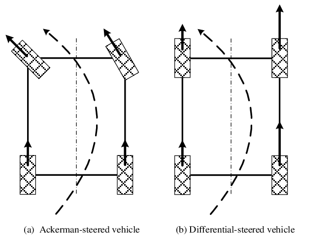
This is important as it will determine where many elements of the robot will go, such as motors, electronics, and our pickup mechanism. The two types of steering we considered were either Ackermann or Differential. Ackermann is familiar to us as we see it in cars, where the back wheels stay at a certain speed and the front wheels can turn. Whereas in differential steering, the back wheels turn at different speeds to turn (i.e., if the left wheel is spinning slower than the right, the robot will turn left).
However, from our understanding and research, Ackermann steering, provided the right geometry and tuning can be much faster than differential steering. With this in mind, we chose differential, while every other team chose Ackermann. This fact definitely made us think about our choice, but those thoughts did not last for long, as we were certain our choice took into consideration that this whole competition was something new to us and we wanted a steering mechanism that we could easily deploy and redeploy. Another observation that pushed us towards this steering mechanism was that the course has some very sharp turns, which in differential steering are easier to control, in just software, rather than in Ackermann steering where you would need to consider the whole chassis layout in order to accomplish those turns.
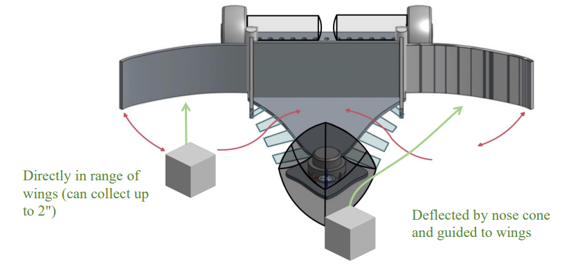
So initially with our constraints, we wanted to design a robot that looked something like this:
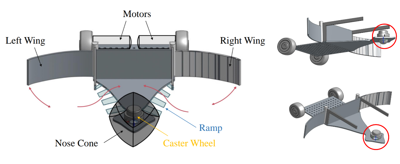
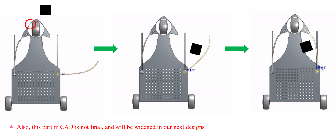
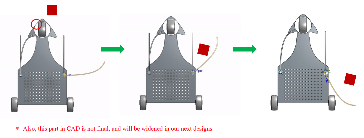
Where we drive around the track, the wings would fold inwards to collect a block and outward to avoid bombs like below:
Construction
Electronics:To start we built a simple line follower, something we could adjust later on. Ebi owned build the motor drivers, tape sensors and microcontroller boards.
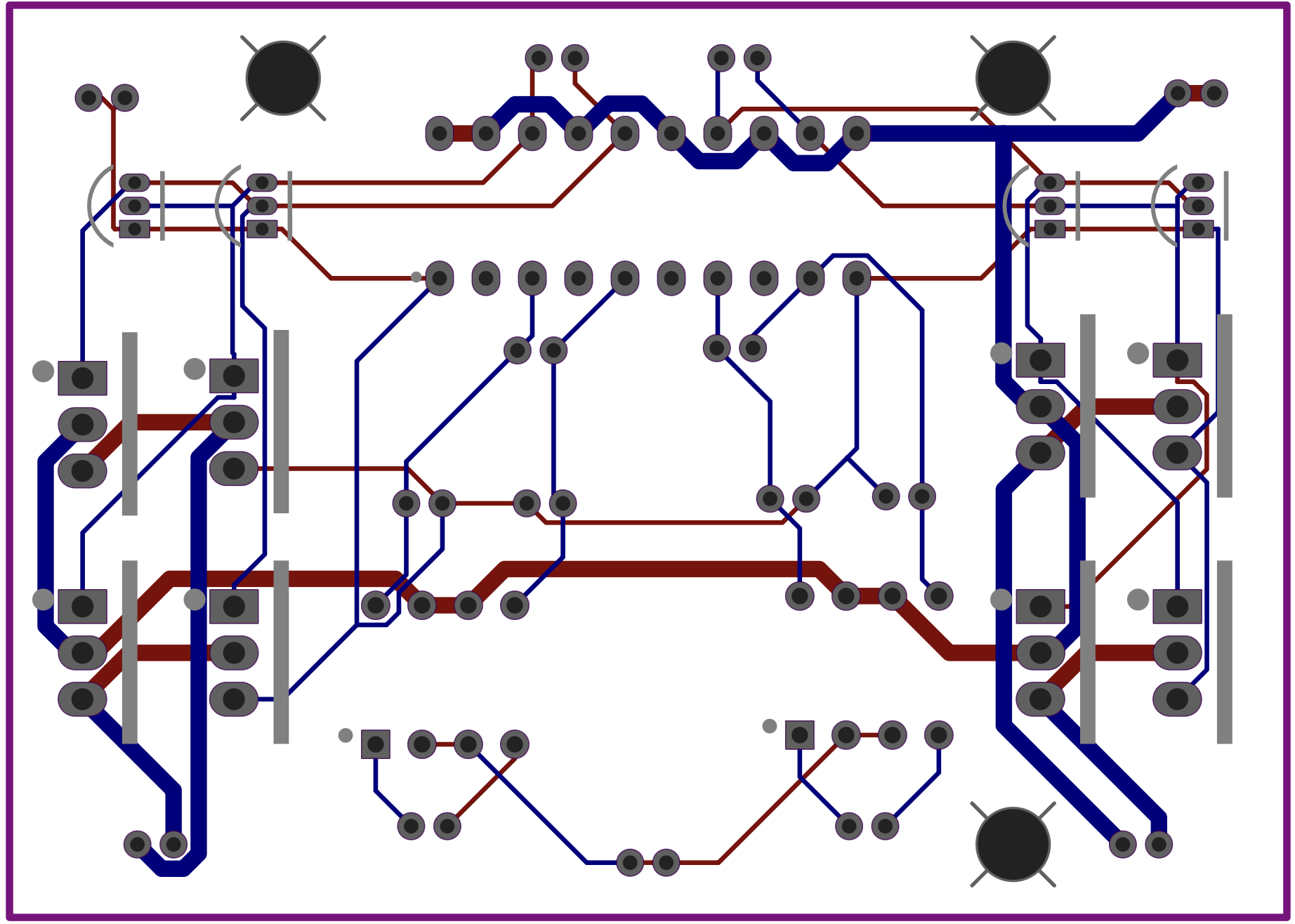
1. H-Bridge Motor Drivers:The H-Bridge is a relatively simple circuit used to control the polarity of the voltage across a load, in our case, a motor. Alongside having control over the speed by PWM, the H-bridge gives us control over the motor’s rotation direction. This is especially important in differential-steering, where in some cases one wheel must spin backward and the other forward to complete a sharp turn. Here is a simple dual H-bridge schematic of the motor boards on the robot.
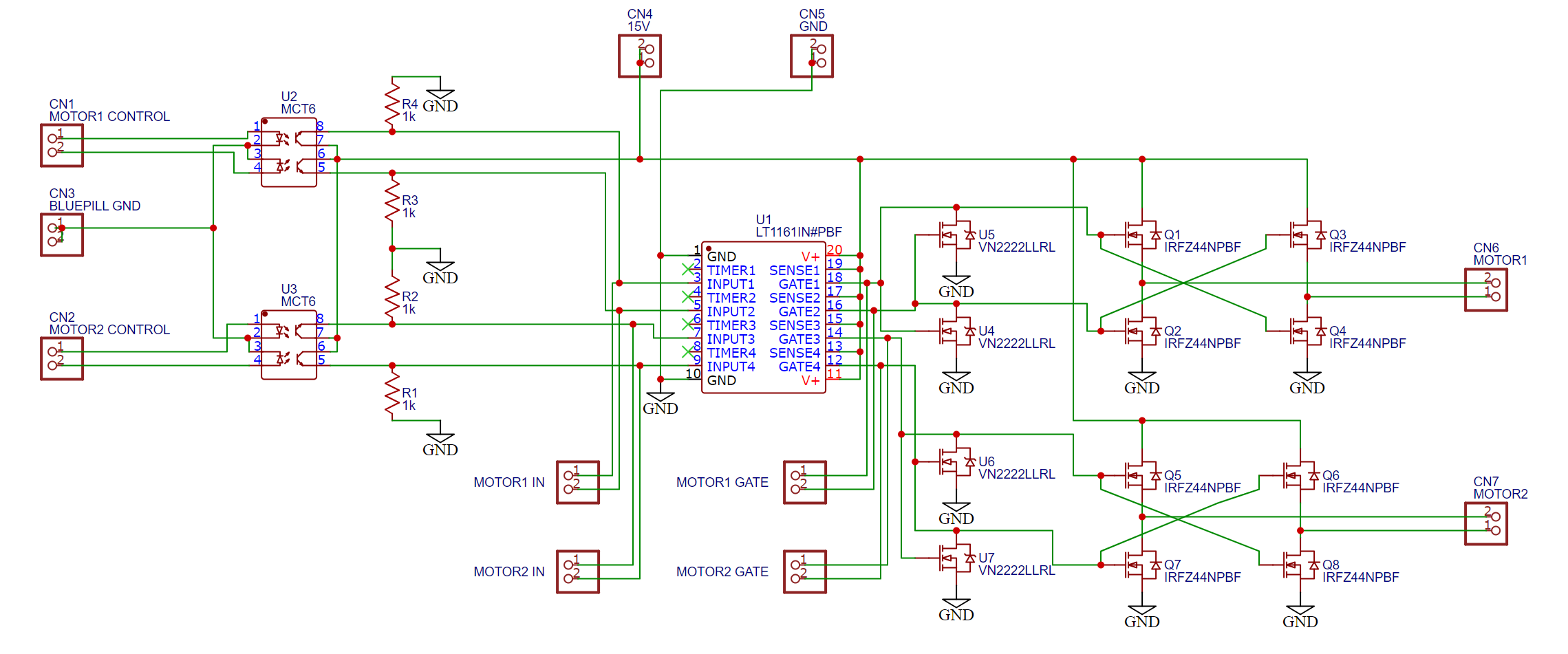
Attached is a step through guide made by Ebi: H-Bridge Step-Through PDF
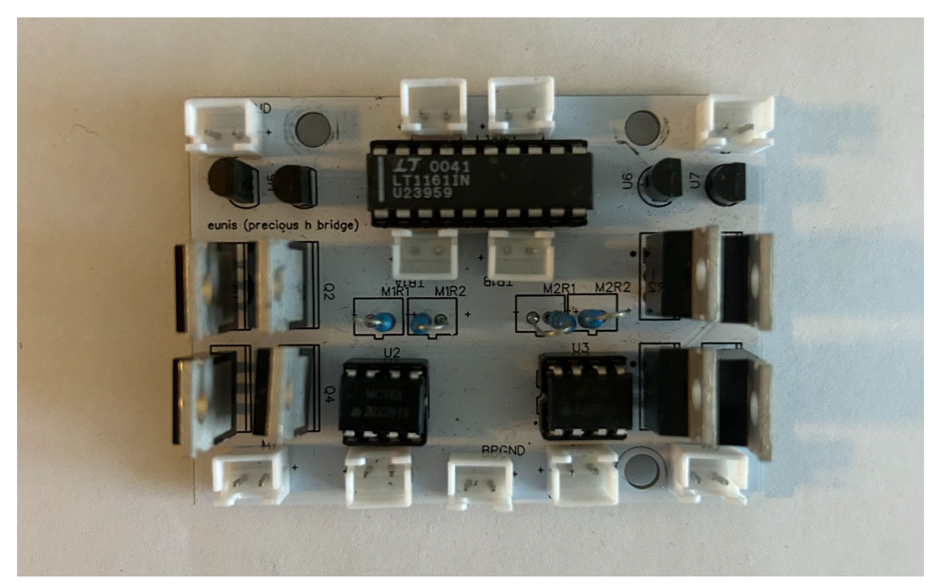
This resulted in:
Here’s the unpopulated Blue-Pill/microcontroller board, and the tape sensor board:
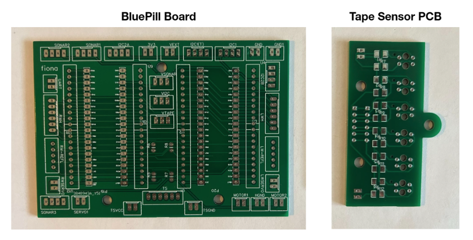
BP Board PCB Layout:
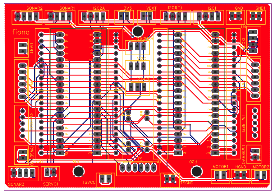
This is somewhat overkill and wasn’t really required in the end, but I designed this board pretty early on before any other sensor / peripheral decisions were made. So it just made sense to be safe and provide the possibility to house two microcontrollers. It has:
- x3 SONAR ports
- x4 I2C ports (two of them tied together if the microcontrollers need to talk to each other)
- x6 AIO available for tape sensors
- x3 servo ports
- a UART port for serial monitor, power selection
- 2 2-wide PWM ports for two H-Bridges
- voltage level selectors for I2C, Sonar, and Tape Sensors
and leaves the remainder of the pins free for switches, LEDS, hall-sensors, and anything else.
For the tape-sensor board, Dhruv made the schematic and Ebi made the PCB layout and soldered it together. It uses surface-mount resistors which was needed since the tape sensors sit very low to the ground. Here’s a video of it on a servo mount which I made using the laser cutter to cut my cad drawings. The black star shaped connector push fit into my mount, for easy prototyping:
The PID is probably the simplest part of code of the entire robot, but I wanted to share how I thought about converting tape-sensor data to an error function.
Instead of computing each sensor value and referencing a lookup table, I decided to treat each sensor value as a force on a seesaw. Then, simply let the displacement be the net torque on it! Of course, if the robot is completely off the line, then just reference the magnitude of the previous displacement to know whether you are too left, or too right.
That’s basically what I’m doing here — writing it in code is much simpler than doing it mathematically though. The key part is the
\[ \sum \frac{S[n]N[n]}{S[n]} \]
You can find the Desmos here, and play around with the ϕ, which is the displacement of the sensor array off the line. The purple line represents the error function value, and the dots are the sensor locations
One interesting way of doing it like this is it becomes convenient to introduce nonlinearities into the transfer function through the R[n] array. Ebi and I played around with this a little and found that a non-linear transfer function for differential steering can often result in smoother and more responsive driving than a linear one.
This makes intuitive sense for tape-following, because you don’t really care about minor deviations off the line, but once your tape sensors are close to leaving the line entirely, you now have a higher error to correct yourself quickly, or to take a sharp turn.
The final “non-traditional” part Ebi and I implemented was filtering the derivative of our error function, so that the PID equation is:
\[ \text{out} = K_p e(t) + K_i \int e(t) \, dt + K_d \cdot \text{lowpass} \left( \frac{d}{dt} e(t) \right) \]
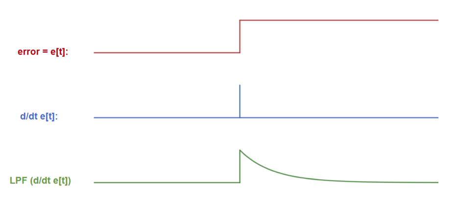
This error function simply means the robot’s displacement off the line has changed. It looks like a step rather than a smooth change because these signals are being processed inside the microcontroller, in the discrete time domain.
If we then compute the almost-discrete-derivative as error - prevErrorerror, we’d get an impulse, as shown in blue. This isn’t that useful because it means the derivative term in the PID equation only lasts for one loop iteration, which is on the order of μs — that’s not nearly enough time for it to do much useful work. A solution to this is to low-pass filter (LPF) the differentiated error signal, shown in green. In an electrical context, this green signal represents the discharging of a capacitor, but instead we’re doing it in software using a first-order IIR filter:
\[ \text{LPF}\left( \frac{d}{dt} e(t) \right) = y(t) = k \cdot y(t - 1) + (1 - k) \left[ e(t) - e(t - 1) \right], \quad k \in (0, 1) \]
Of course there are other ways to do this, and I guess you could choose any decaying function (maybe an average?). All that I’m trying to do is keep the effect of the derivative for longer, so that the KdKd term comes into play.
The motivation to try something like this is somewhat arbitrary, but we gave it a shot and it had a significant positive impact on the smoothness of the robot’s tape following at high speeds.
Final run:With all the basics sorted, we put the motors, H-bridges, microcontrollers, tape-sensors, and PID code together for the first prototype. Here you can see one of the populated BP boards as well.
I’m really proud of the pace we were able to do this at, since we were the first team to get on the track and tape follow in the first week of the course.
We fail on rainbow road since this was our first time testing, and the colors interfered with the tape sensor
Final Build
Here is a demonstration of a ~16 second lap, our final design:
UBC EngPhys Robot Summer 2023